<women.R>
library(rstan)
data(women)
attach(women)
x <- women$weight
y <- women$height
N <- nrow(women)
model_A <- glm(formula = y~x, data =women)
plot(x,y)
abline(model_A,col='red', lty=1)
data_stan <-list(x=x, y=y, N=N)
Linear_model <-stan(file="women.stan", data=data_stan, iter = 2000, warmup = 1000, chains = 4)
q_model <-stan(file="women_sq.stan", data=data_stan, iter = 2000, warmup = 1000)
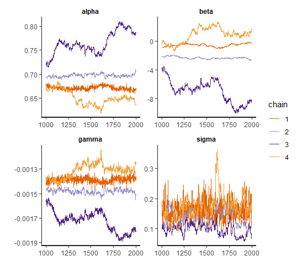
traceplot(q_model,inc_warmup=FALSE)
수렴이 안되기 때문에 개선이 필요하다.
<women.stan>
data {
int<lower=0> N; #number of observation, 관찰수
vector[N] x; #predictor,예측변수
vector[N] y; #response variable, 응답변수
}
transformed data{
vector[N] x_sq; # transformed data as squared of the weight
x_sq <- x .*x; #formula for the transformation
}
parameters {
real alpha; # 기울기, slope parameter,실수
real beta; # 절편, intercept parameter
real gamma; #parameter for the weight squared
real<lower=0> sigma;#표준편차, standard deviation,양수
}
model {
y ~ normal(alpha*x + gamma*x_sq + beta, sigma); //likelihood
}
iter 를 증가시커나 stepsize를 작게 만들어야 된다.
q_model <-stan(file="women_sq.stan", data=data_stan, iter = 7000, control=list(stepsize=0.0001))
traceplot(q_model,inc_warmup=FALSE)


print(q_model)
|
|
mean
|
se_mean
|
sd
|
2.50%
|
25%
|
50%
|
75%
|
97.50%
|
n_eff
|
Rhat
|
|
alpha
|
0.84
|
0
|
0.03
|
0.78
|
0.82
|
0.84
|
0.86
|
0.9
|
224
|
1.01
|
|
beta
|
-12.02
|
0.13
|
1.95
|
-16.07
|
-13.19
|
-11.95
|
-10.87
|
-8.17
|
225
|
1.01
|
|
gamma
|
0
|
0
|
0
|
0
|
0
|
0
|
0
|
0
|
224
|
1.01
|
|
sigma
|
0.08
|
0
|
0.02
|
0.05
|
0.07
|
0.08
|
0.09
|
0.14
|
217
|
1.03
|
|
lp__
|
28.56
|
0.11
|
1.87
|
23.6
|
27.73
|
29.03
|
29.89
|
30.72
|
303
|
1.01
|
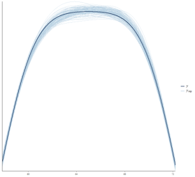
복제 데이터로 학습
Stan에 복제데이터 추가
generated quantities{
real y_rep[N]; #replicated data
for(i in 1:N){
y_rep[i] = normal_rng(alpha*x[i] + gamma*x_sq[i] + beta,sigma);
}
}
Stan학습
q_model_rep <-stan(file="women_sq_rep.stan", data=data_stan, iter = 9000, control=list(stepsize=0.00001))
traceplot(q_model_rep,inc_warmup=FALSE)
print(q_model_rep)
y_rep <-as.matrix(q_model_rep, pars = "y_rep")

그래프로 확인
library(bayesplot)
dim(y_rep)
head(y_rep[1:3,],4)
ppc_dens_overlay(y,yrep=y_rep[1:100,])
모델진단
Plot으로 수렴확인
class(Linear_model) #출력은 stanfit과 rstan
posterior <-extract(Linear_model)
par(mfrow=c(1,3))
plot(posterior$alpha,type="l",main="Alpha")
plot(posterior$beta,type="l",main="Beta")
plot(posterior$sigma,type="l",main="Sigma")
@posterior는 alpha,beta,sigma,lp_ 변수로 구성
@extract는 rstan패키지함수임

model_bad <-stan(file="women.stan", data=data_stan, iter = 50, warmup = 25)
post_bad <-extract(model_bad)
par(mfrow=c(1,3))
plot(post_bad$alpha,type="l",main="Alpha")
plot(post_bad$beta,type="l",main="Beta")
plot(post_bad$sigma,type="l",main="Sigma")

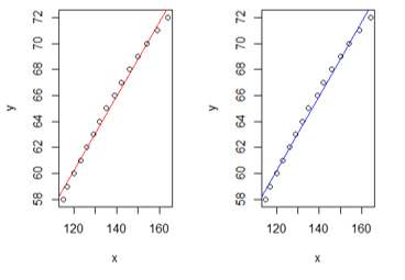
Plot the Fit both Bayesian and Non Bayesian
par(mfrow = c(1,2))
plot(x,y)
abline(model_A, col="red",lty=1)
plot(x,y)
abline(mean(posterior$beta),mean(posterior$alpha),col="blue")
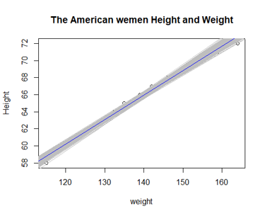
plot(x,y, main="The American wemen Height and Weight", xlab = "weight", ylab = "Height")
for(i in 1:500){
abline(mean(posterior$beta[i]),mean(posterior$alpha[i]),
col="grey",lty=1)
}